Overview

Gradient descent is an optimization algorithm which is commonly used in machine learning, it is a technique to find the minimum value of a function.

Mathematic Basics

Derivative

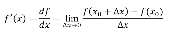
For single-variable function f(x), derivative is the slope of tangent line at one point, which represents the rate of change of the function at that point. As shown below, the function's derivative at x = x₀ is (if ∆x→0 exists, this conditions shall not be restated hereafter):

Tangent line to a plane curve at a given point is the straight line that 'just touches' the curve at that point, and the direction of the tangent line is the same as the point.

Partial Derivative

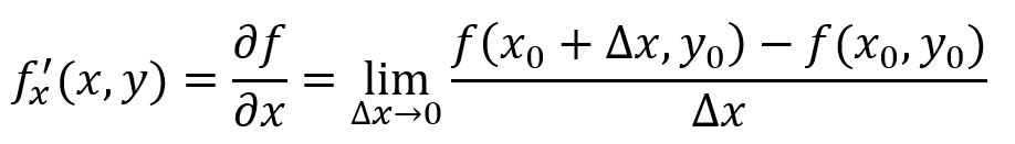
It is much more complicated when it comes to multiple-variable functions. If we only consider the change of one variable but keep other variables unchanged, we would get a partial derivative of the function. A function with N variables have N partial derivatives. For instance, function f(x,y) 's partial derivative at x = x₀ is:

In figure above, L1 represents the change of the function along the Y-axis, i.e., the derivative of y when treating x as constant; L2 represents the change of the function along the X-axis, i.e., the derivative of x when treating y as constant.

Directional Derivative

Derivative and partial derivative consider function's changes in the direction of axes. If to consider function's changes in any direction, it is directional derivative.

Taking two-variable function z = f(x,y) as an example, for any point (x₀,y₀,z₀) on the function's curved surface, its projection on the XY plane is point (x₀,y₀). Draw a unit circle with (x₀,y₀) as the center of the circle, the unit vector (denoted as u) formed by any point on the circle and (x₀,y₀) can express direction. In particular, when the direction coincides with the positive direction of the coordinate axis, directional derivative is partial derivative.

Gradient

The direction in which the function value rises the fastest, that is, the direction in which the directional derivative obtains the maximum value, is the direction of the gradient. Conversely, the function value decreases most rapidly in the opposite direction to the gradient.

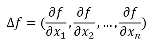
Directional derivative in any direction is linear combination of partial derivatives. It has been proven that the gradient (denoted ∇f) of the multi-variable function f(x1,x 2,...,xn) is

Chain Rule

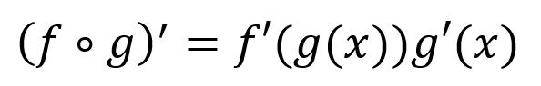
Chain rule states that the derivative of composite function can be expressed as the product of the derivatives of the individual functions that make up the composite function. The mathematical expression is: for compositive function f∘g, its derivative is:

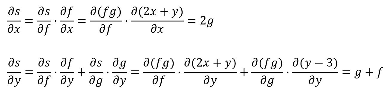
For instance, composite function s(x,y) = (2x+y)(y-3) is composed of f(x,y) = 2x+y and g(y) = y-3, thus s(x,y)'s partial derivatives for x and y are：

Gradient Descent

Basic Form

Take a real-life example: let's say we are on a mountain and wish to go down as fast as possible. Of course, there must be a best route, but usually it is costly to find that very path. It is more common to take one step at a time. In another word, each time we reach a new position, calculate the direction (gradient) in which we can go down the fastest, and go to the next position in that direction. Repeat this process until we reach the foot of the mountain.

Gradient descent is the method to find the minimum value in the direction of gradient descent; finding the maximum value in the direction of gradient ascent, on the other hand, is the method of gradient ascent.

Given a function J(θ), the basic form of gradient descent is:

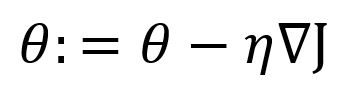
where ∇J is the gradient of function at the position of θ, η is the learning rate. As gradient is actually the quickest direction the function value ascends, the minus before η∇J represents the opposite direction of gradient.

Learning rate is the length of each movement on gradient descending direction towards the target. In example above, learning rate can be understood as the length of each step we take.

Single-Variable Function Example

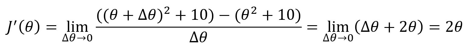
Taking function J(θ) = θ² + 10 as example, the derivative is:

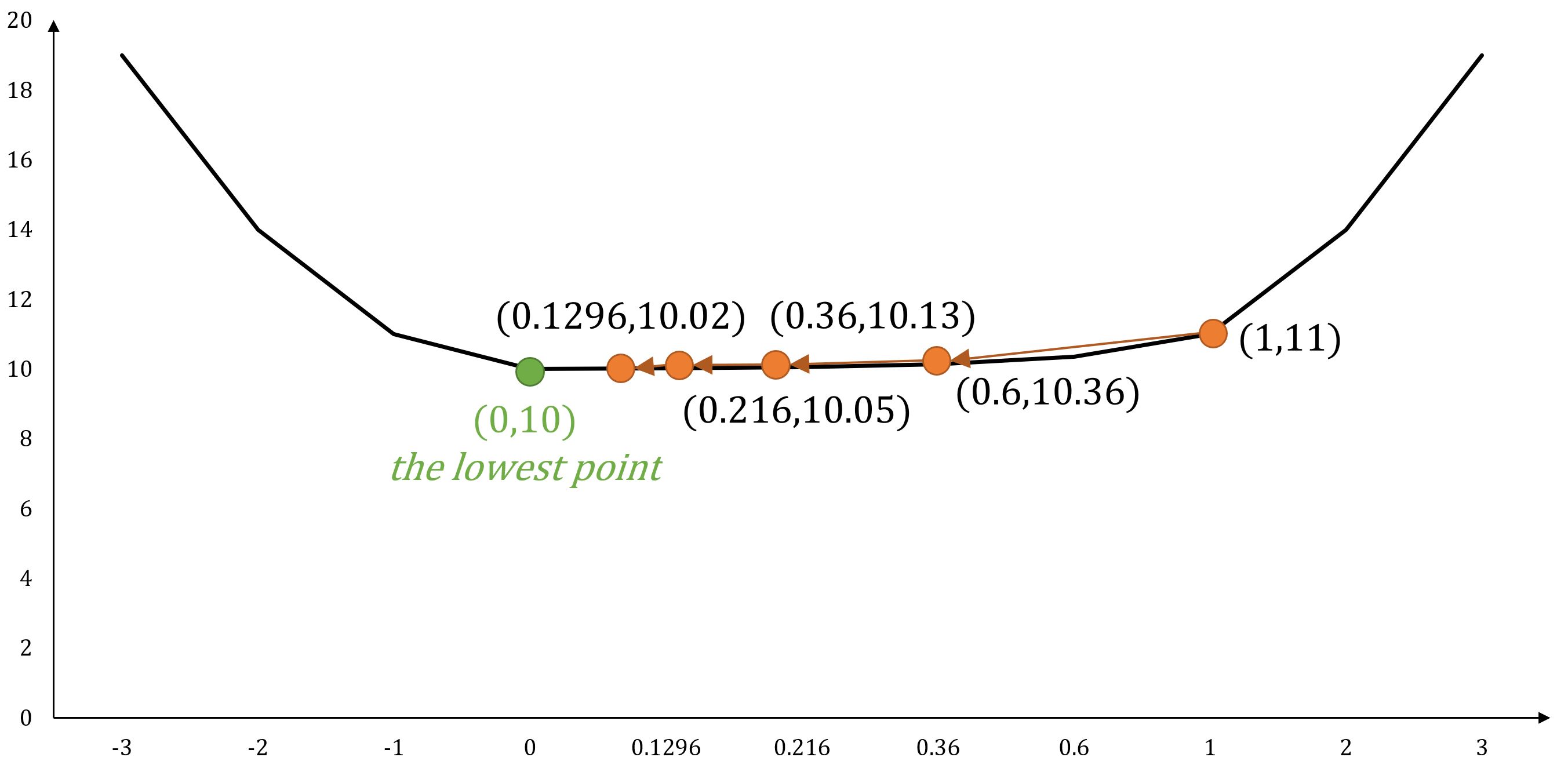
If starts from position θ₀ = 1, with learning rate η = 0.2, based on the gradient descent formula, the next movements would be:

• θ₁ = 1 - 2*1*0.2 = 0.6
• θ₂ = 0.36
• θ₃ = 0.216
• θ₄ = 0.1296
• ...
• θ₁₈ = 0.00010156
• ...

With the number of steps increasing, we infinitely approach position θ = 0 which brings the minimum value of the function.

Multi-Variable Function Example

Taking J(Θ) = θ₁² + θ₂² as example, the derivatives are:

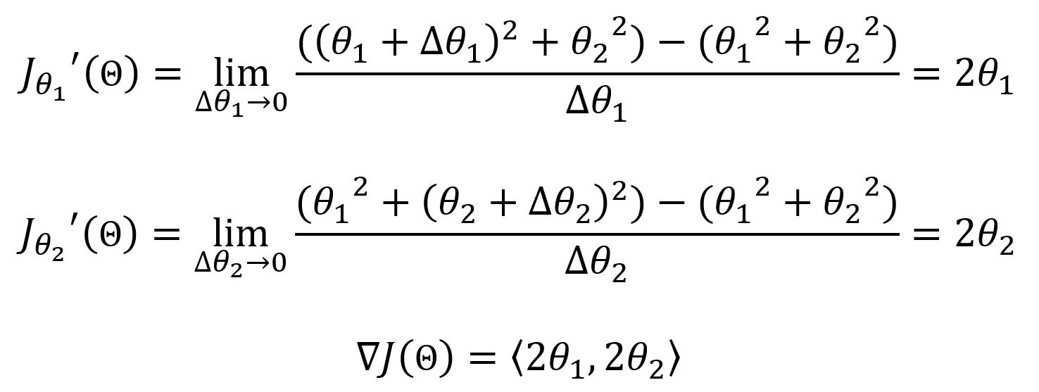
If starts from position Θ₀ = (-1,-2), with learning rate η = 0.1, based on the gradient descent formula, the next movements would be:

• Θ₁ = ((-1) - 2*(-1)*0.1,(-2) - 2*(-2)*0.1) = (-0.8,-1.6)
• Θ₂ = (-0.64,-1.28)
• Θ₃ = (-0.512,-1.024)
• Θ₄ = (-0.4096,-0.8192)
• ...
• Θ₂₀ = (-0.011529215,-0.02305843)
• ...

With the number of steps increasing, we infinitely approach position Θ = (0,0) which brings the minimum value of the function.

Gradient Descent in Machine Learning

In the learning and training of neural network model, a loss/cost function J(Θ) is often employed to evaluate the error between output of the model and the expected result, gradient descent technique is then used to minimize this loss function, i.e, repetitively updating the parameters of the model in the opposite direction of gradient ∇J(Θ) until convergence so as to optimize the model. For the balance of computation time and accuracy, there are some variant forms of gradient descent that have been used in practices, including:

1. Batch Gradient Descent, BGD
2. Stochastic Gradient Descent, SGD
3. Mini-Batch Gradient Descent, MBGD

Example Description

Assume that we are using m samples to train a neural network model; sample often refers to a group of input value and expected output, and x⁽ⁱ⁾ and y⁽ⁱ⁾ (i=1,2,...,m) are the i-th input value and the i-th expected output. The hypothesis h_Θ of the model is as below, where the subscripts of x⁽ⁱ⁾ represents x⁽ⁱ⁾'s components:

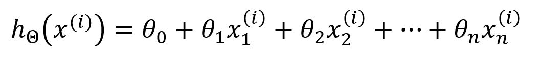
Hypothesis is a target function that describes the mappings of inputs to outputs in machine learning. In this example, any change to the parameter θ_j (j=0,1,...,n) would result in changes to the outputs of the model. The goal of model training is to find the optimal θ_j that makes the outputs to be as close as possible to the expected values. In the beginning of the training, θ_j is randomly initialized.

Let's use the mean square error (MSE) as the loss/cost function J(Θ) to describe the average error between each expected value and the output:

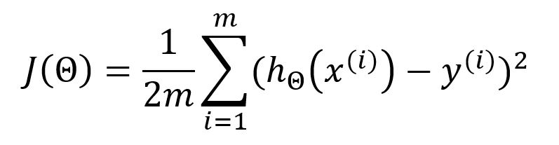
Denominator in the standard MSE is 1/m, 1/2m is used in machine learning instead to offset the square when the loss function is derived, constant coefficient is thus eliminated for the convenience of subsequent calculations. The results will not be affected in this way.

Batch Gradient Descent

Batch gradient descent (BGD) is the original form of gradient descent.

Calculate partial derivative for θ_j:

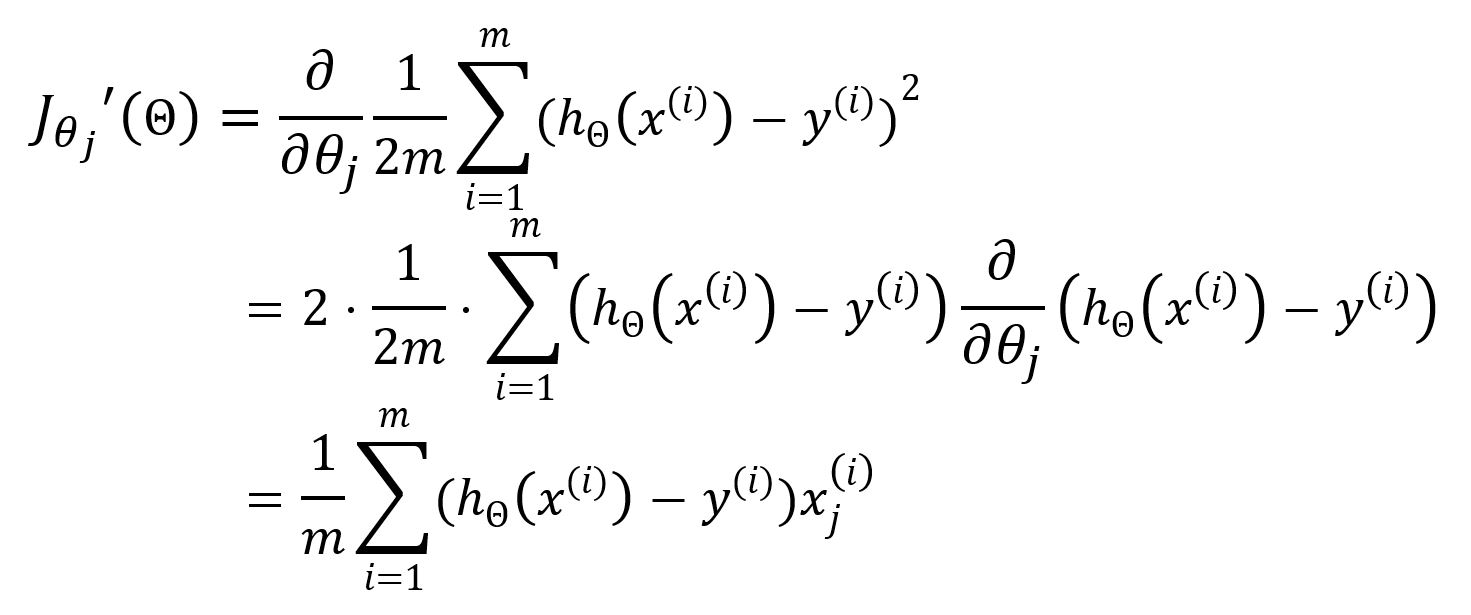
Update θ_j:

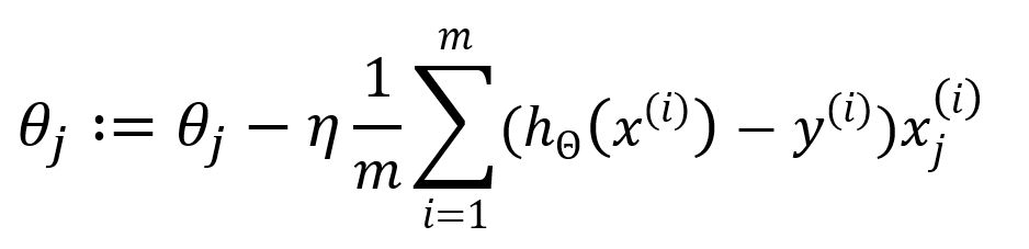
where η is the learning rate. The sum symbol shows that all m samples will participate in each iteration to update the parameters. Obviously, the training process will be slow when m is considerable large.

Stochastic Gradient Descent

Stochastic gradient descent (SGD) is theoretically similar to BGD, while SGD selects only one sample for each iteration to speed up the training process.

Select one sample randomly to calculate error:

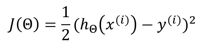
Calculate partial derivatives for θ_j:

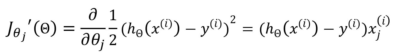
Update θ_j:

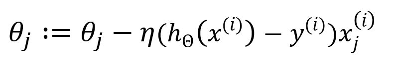
The computation complexity is reduced because SGD uses only one sample and skips the process of summation and averaging, computation speed is improved with the cost of some accuracy.

Mini-Batch Gradient Descent

The two methods above both take extremes, either they involve all samples or only one sample. Mini-batch gradient descent (MBGD) serves as a compromise approach by selecting 1 < x < m samples randomly to perform the computation.