Gradient Descent

Gradient descent is a fundamental optimization algorithm widely used in graph embedding models. Its primary purpose is to iteratively update model parameters in order to minimize a predefined loss/cost function.

To handle the computational challenges of large-scale graph embedding, several variants of gradient descent have been developed. Two commonly used ones are Stochastic Gradient Descent (SGD) and Mini-Batch Gradient Descent (MBGD). These variations update model parameters using gradients computed from either a single data point or a small subset of data during each iteration.

Basic Form

Consider a real-life scenario: standing on a mountain and aiming to descend as quickly as possible. While there may be an optimal path, identifying if in advance is difficult. Instead, a step-by-step approach is used—at each position, you assess the steepest downward direction and take a step accordingly. At each iteration, the algorithm calculates the direction that minimizes the loss most rapidly (the gradient) and updates the parameters accordingly. The process continues until the minimum (the base of the mountain) is reached.

Building on this concept, gradient descent serves as the technique to find the minimum of a function by moving in the direction of the negative gradient. Conversely, if the goal is to find a maximum, the algorithm follows the positive gradient direction, a technique known as gradient ascent.

along the gradient's descent. Conversely, if the aim is to locate the maximum value while ascending along the gradient's direction, the approach becomes gradient ascent.

Given a function $J(\theta )$, the basic form of gradient descent is:

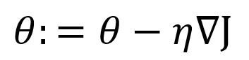
where $\nabla J$ is the gradient of the function at the position of $\theta$, $\eta$ is the learning rate. Since gradient is the steepest ascent direction, a minus symbol is used before $\eta \nabla J$ to get the steepest descent.

The learning rate determines the step size taken in the direction of the gradient during optimization. In the example above, the learning rate corresponds to the distance covered in each step during the descent.

The learning rate is typically kept constant throughout the training process, where the rate is adjusted over time—often decreased gradually or according to a predefined schedule. Such adjustments are designed to improve convergence stability and optimization efficiency.

Example: Single-Variable Function

For function $J={\theta }^2+10$, its gradient (in this case, same as the derivative) is $\nabla J=J\prime (\theta )=2\theta$.

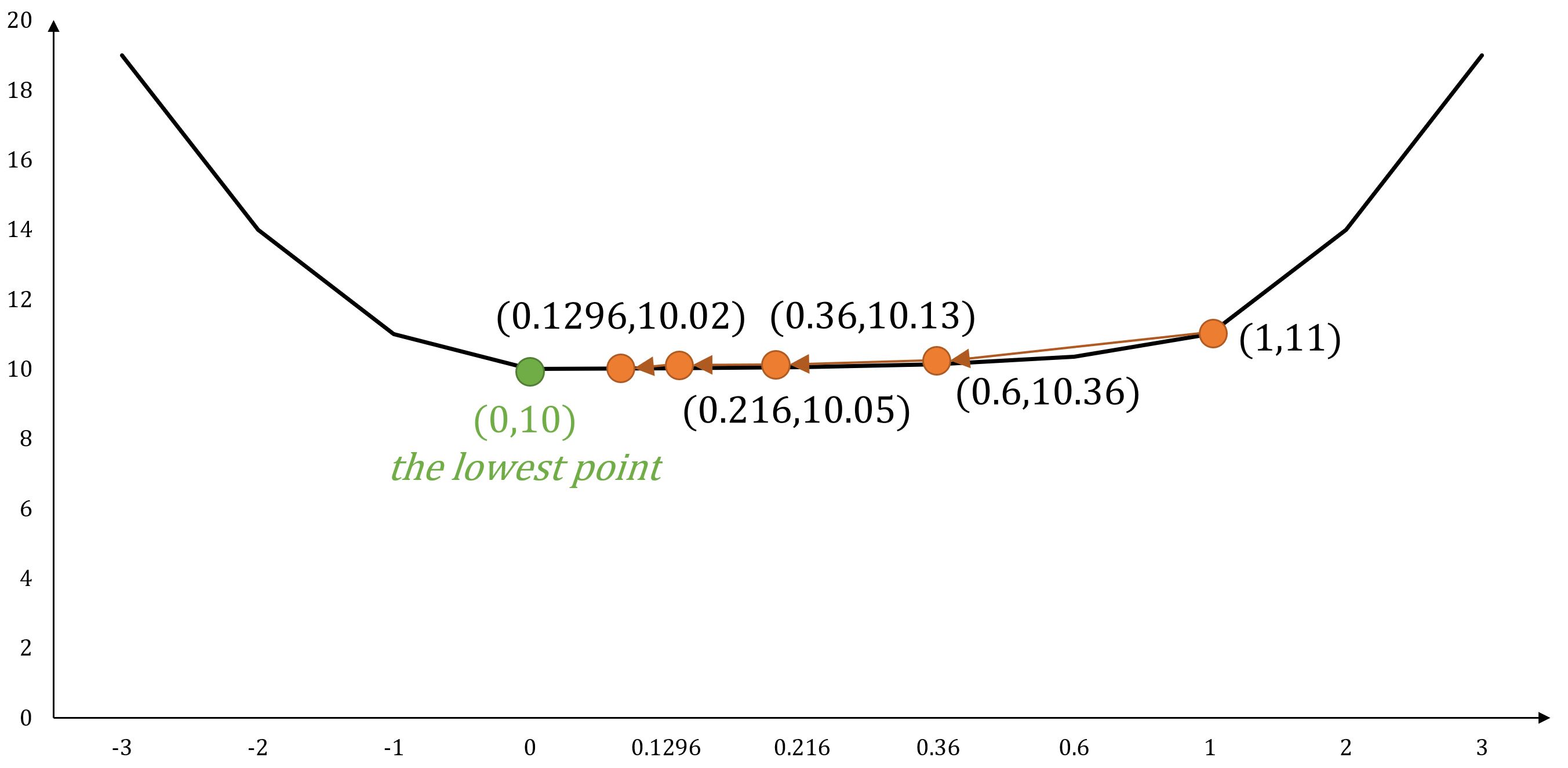
If we start at position ${\theta }_0=1$, and set $\eta =0.2$, the next movements following gradient descent would be:

• ${\theta }_1={\theta }_0-\eta \times 2{\theta }_0=1-0.2\times 2\times 1=0.6$
• ${\theta }_2={\theta }_1-\eta \times 2{\theta }_1=0.6-0.2\times 2\times 0.6=0.36$
• ${\theta }_3={\theta }_2-\eta \times 2{\theta }_2=0.36-0.2\times 2\times 0.36=0.216$
• ...
• ${\theta }_{18}=0.00010156$
• ...

As the number of steps increases, the process gradually converges toward $\theta =0$, ultimately reaching the minimum of the function.

Example: Multi-Variable Function

For function $J(\Theta )={\theta }_1^2+{\theta }_2^2$, its gradient is $\nabla J=(2{\theta }_1\mathrm{, }2{\theta }_2)$.

If starts at position ${\Theta }_0=(-1\mathrm{, }-2)$, and set $\eta =0.1$, the next movements following gradient descent would be:

• ${\Theta }_1=(-1-0.1\times 2\times -1\mathrm{, }-2-0.1\times 2\times -2)=(-0.8\mathrm{, }-1.6)$
• ${\Theta }_2=(-0.64\mathrm{, }-1.28)$
• ${\Theta }_3=(-0.512\mathrm{, }-1.024)$
• ...
• ${\Theta }_{20}=(-0.011529215\mathrm{, }-0.002305843)$
• ...

As the number of steps increases, the process gradually converges toward $\Theta =(0\mathrm{, }0)$, ultimately reaching the minimum of the function.

Application in Graph Embeddings

In the process of training a neural network model for graph embeddings, a loss or cost function, typically denoted as $J(\Theta )$, is used to assess the discrepancy between the model's output and the expected outcomes. To minimize this loss, gradient descent is used. This iterative optimization technique updates the model's parameters in the opposite direction of the gradient $\nabla J$. This process continues until the model converges to a minimum, thereby optimizing performance.

To balance computational efficiency and model accuracy, several variants of gradient descent are commonly used in practice, including:

1. Stochastic Gradient Descent (SGD)
2. Mini-Batch Gradient Descent (MBGD)

Example

Consider a scenario where we are training a neural network model using a set of $m$ samples. Each sample consists of an input value and its corresponding expected output. Let's use $x^{(i)}$ and $y^{(i)}$ ($i=1\mathrm{, }2\mathrm{, }\mathrm{...}\mathrm{, }m$) denote the input and expected output of the $i$-th sample.

The hypothesis $h(\Theta )$ of the model is defined as:

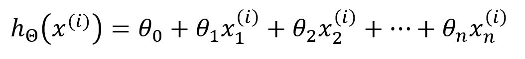
Here, $\Theta$ represents the model's parameters ${\theta }_0$ ~ ${\theta }_n$, and $x^{(i)}$ is the $i$-th input vector, consisting of $n$ features. The model computes the output using a function $h(\Theta )$, which performs a weighted combination of the input features.

The objective of model training is to identify the optimal values of ${\theta }_{\mathrm{j}}$ that produce outputs as close as possible to the expected values. At the beginning of training, ${\theta }_{\mathrm{j}}$ is initialized with random values.

During each iteration of model training, after computing the outputs for all samples, the mean squared error (MSE) is used as the loss/cost function $J(\Theta )$. It measures the average squared difference between the predicted output and its corresponding expected value:

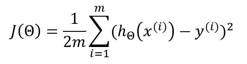
In the standard MSE formula, the denominator is usually $\frac{1}{m}$. However, $\frac{1}{2m}$ is often used instead to offset the squared term when taking the derivative. This leads to the elimination of the constant coefficient during gradient calculation, simplifying subsequent computations without affecting the final result.

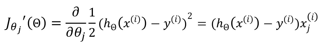
Subsequently, gradient descent is used to update the parameters ${\theta }_j$. The partial derivative of the loss function with respect to ${\theta }_j$ is calculated as follows:

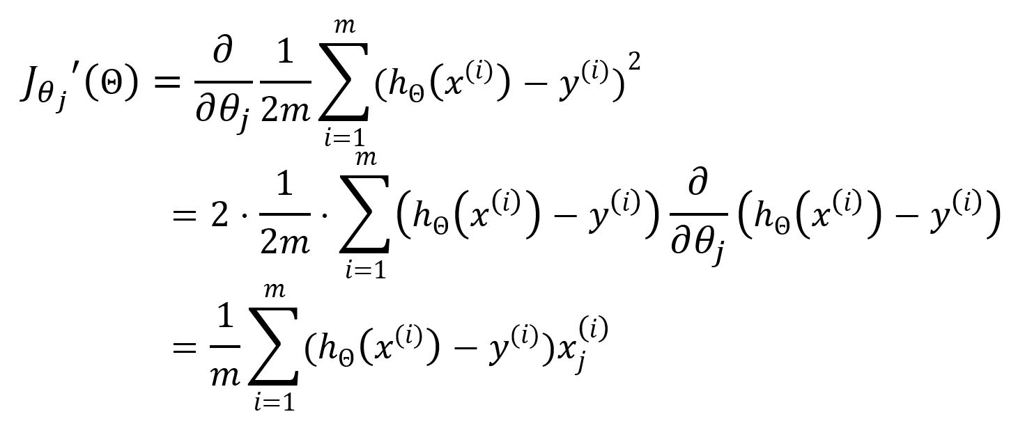
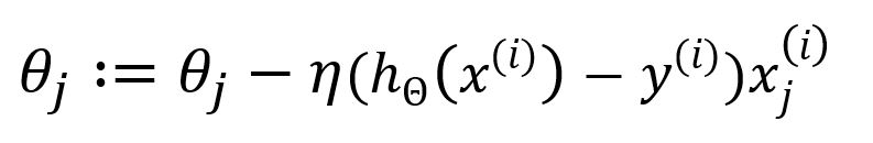
Hence, update ${\theta }_j$ as:

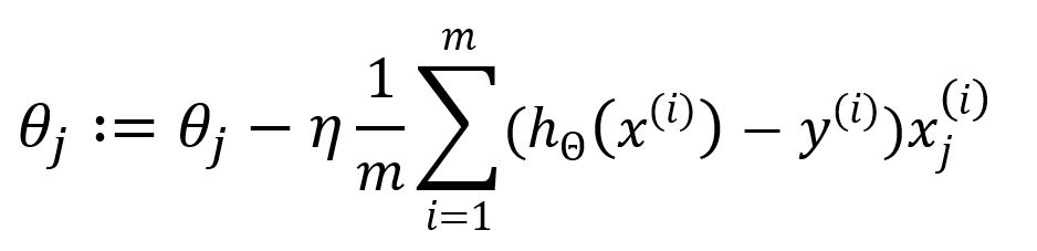
The summation from $i=1$ to $m$ indicates that all $m$ samples are used in each iteration to update the parameters. This approach is known as Batch Gradient Descent (BGD), the original and most straightforward form of the gradient descent algorithm. In BGD, the entire sample dataset is used to compute the gradient of the cost function during each iteration.

While BGD offers precise convergence to the minimum of the cost function, it can be computationally intensive for large datasets. To improve efficiency and convergence speed, SGD and MBGD were introduced. These variants use subsets of the data in each iteration, significantly accelerating the optimization process while still aiming to find the optimal parameters.

Stochastic Gradient Descent

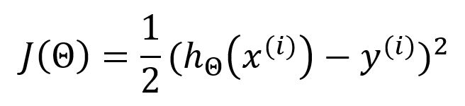
Stochastic gradient descent (SGD) only selects one sample in random to calculate the gradient for each iteration.

When employing SGD, the above loss function should be expressed as:

The partial derivative with respect to ${\theta }_j$ is:

Update ${\theta }_j$ as:

SGD reduces computational complexity by using only one sample per iteration, eliminating the need for summation and averaging. This leads to faster computation but may sacrifice some accuracy in the gradient estimation.

Mini-Batch Gradient Descent

BGD and SGD both represent two extremes: BGD uses all samples, while SGD uses only one. Mini-batch Gradient Descent (MBGD) strikes a balance by randomly selecting a subset of $x\in (1\mathrm{, }m)$ samples for computation.

Mathematical Basics

Derivative

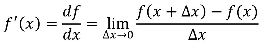
The derivative of a single-variable function $f(x)$ is often denoted as $f\prime (x)$ or $\frac{df}{dx}$, it represents how $f(x)$ changes with respect to a slight change in $x$ at a given point.

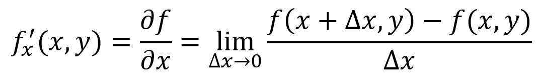
Graphically, $f\prime (x)$ corresponds to the slope of the tangent line to the function's curve. The derivative at point $x$ is:

For example, $f(x)=x^2+10$, at point $x=-7$:

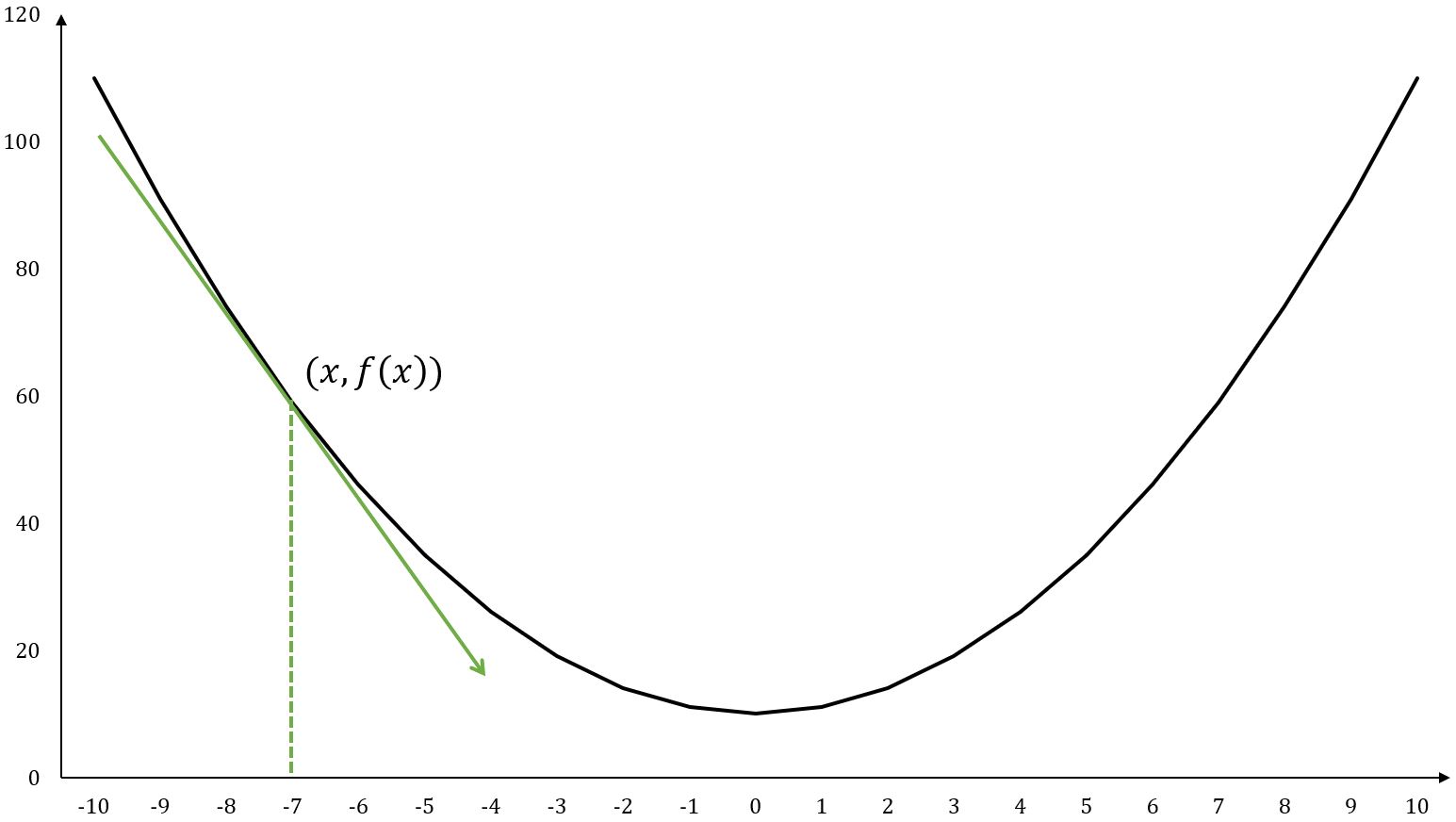
A tangent line is a straight line that touches a function's curve at exactly one point and has the same slope (direction) as the curve at that point.

Partial Derivative

The partial derivative of a multiple-variable function measures how the function changes as one specific variable changes, while all other variables are held constant. For a function $f(x,y)$, its partial derivative with respect to $x$ at a particular point $(x,y)$ is denoted as $\frac{\partial f}{\partial x}$ or $f_x^{\prime }$:

For example, $f(x,y)=x^2+y^2$, at point $x=-4$, $y=-6$:

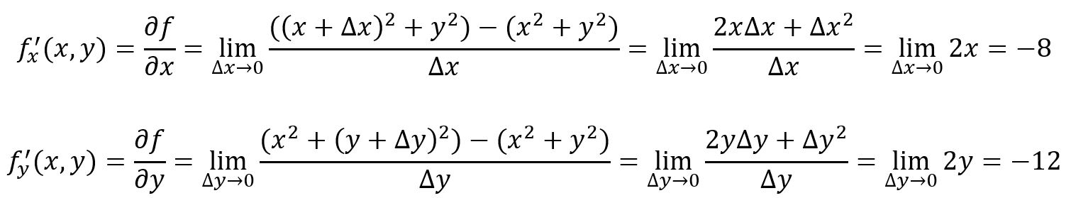
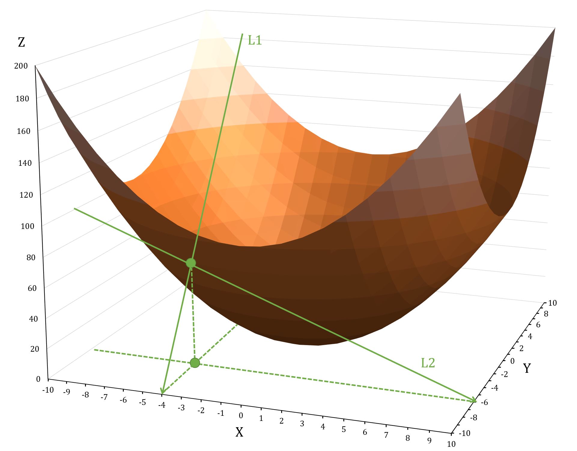
$L1$ shows how the function changes as you move along the Y-axis, while keeping $x$ constant; $L2$ shows how the function changes as you move along the X-axis, while keeping $y$ constant.

Directional Derivative

The partial derivative of a function describes how its output changes when moving slightly along one of the coordinate axes. However, when movement occurs in a direction that is not parallel to any axis, the concept of the directional derivative becomes crucial.

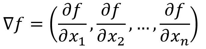
The directional derivative is mathematically expressed as the dot product of the vector $\nabla f$ composed of all partial derivatives of the function with the unit vector $\overrightarrow{w}$ which indicates the direction of the change:

where $|\overrightarrow{w}|=1$, $\theta$ is the angle between the two vectors, and

Gradient

The gradient shows the direction in which a function increases the fastest. This is the same as finding the maximum directional derivative. This occurs when angle $\theta$ between the vectors $\nabla f$ and $\overrightarrow{w}$ is $0$, as $\cos 0=1$, implying that $\overrightarrow{w}$ aligns with the direction of $\nabla f$. $\nabla f$ is thus called the gradient of a function.

Naturally, the negative gradient points in the direction of the steepest descent.

Chain Rule

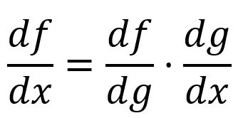
The chain rule describes how to calculate the derivative of a composite function. In the simpliest form, the derivative of a composite function $f(g(x))$ can be calculated by multiplying the derivative of $f$ with respect to $g$ by the derivative of $g$ with respect to $x$:

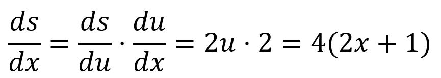
For example, $s(x)={(2x+1)}^2$ is composed of $s(u)=u^2$ and $u(x)=2x+1$:

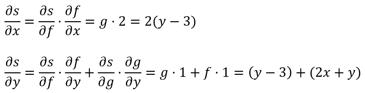
In a multi-variable composite function, the partial derivatives are obtained by applying the chain rule to each variable.

For example, $s(x,y)=(2x+\mathrm{y})(y-3)$ is composed of $s(f,g)=fg$ and $f(x,y)=2x+\mathrm{y}$ and $g(x,y)=y-3$: