Overview

Many seasoned users of traditional databases and data frameworks find themselves at a crossroads when transitioning from a familiar relational database to the realm of graph databases. The time and effort invested in learning graph query commands do not necessarily ease this early challenge of seamlessly migrating data to a graph database.

For users grappling with the complexity of managing hundreds of data fields scattered across numerous relational tables, the task of data migration proves to be an incredibly daunting challenge:

• Inappropriate Distinction of Nodes and Edges

The nomenclature of data tables often presents all tables as distinct entities in the real world. This can lead to confusion when users try to discern which tables represent authentic entities and which ones depict relationships between these entities.

• Excessive Redundant Fields Lingering in Schemas

The idea of 'redundant fields,' intended for addressing the inefficiency of SQL’s table JOIN queries, lingers in users' minds. This makes the removal or replacement of these fields challenging, especially when dealing with the design of graph data.

• Insufficient Restructuring of the Table Framework

After numerous iterations of modifications to the table structures, the final graph model may, at times, deviate significantly from the original table structure. Embarking on such major transformation is a task very few beginners are willing to undertake.

Blurt out Truth

Whether the user's data is structured in tables or not, it often cannot be directly converted into graph data. Graph data adheres to specific requirements: nodes must possess unique IDs serving as their identity cards, while edges must have designated FROM and TO, both referencing node IDs within the graph. Only then can we truly appreciate the beauty of an edge, "a magnificent bridge linking nodes together!"

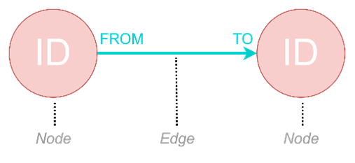
An illustration of node’s ID and edge’s FROM, TO

This arduous data migration journey usually involves numerous rounds of fine tuning data schemas[1]. If there were any golden rules or sacred principles in this battle of data transformation, they would be: meticulously focus on the primary keys and foreign keys within the original tables. These keys will become the IDs for nodes and the FROM and TO for edges, making them the pivotal elements for successfully obtaining graph data.

Let's delve into a practical example demonstrating how to transform the table structure of a Hospital Information Management System built using SQL Server into a graph model and then import the resulting graph data into an Ultipa graph system. 

In simplifying matters, consider this Hospital Information Management System holding fundamental details about doctors, patients, departments, and hospital beds, alongside records of doctors' consultations and patients' hospitalizations. All these data are stored across six distinct tables:

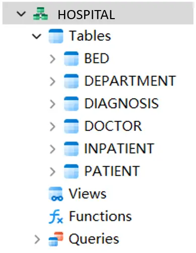Tables created for a hospital information management system in SQL Server

Let's create a diagram to visually depict the relationships among these tables:

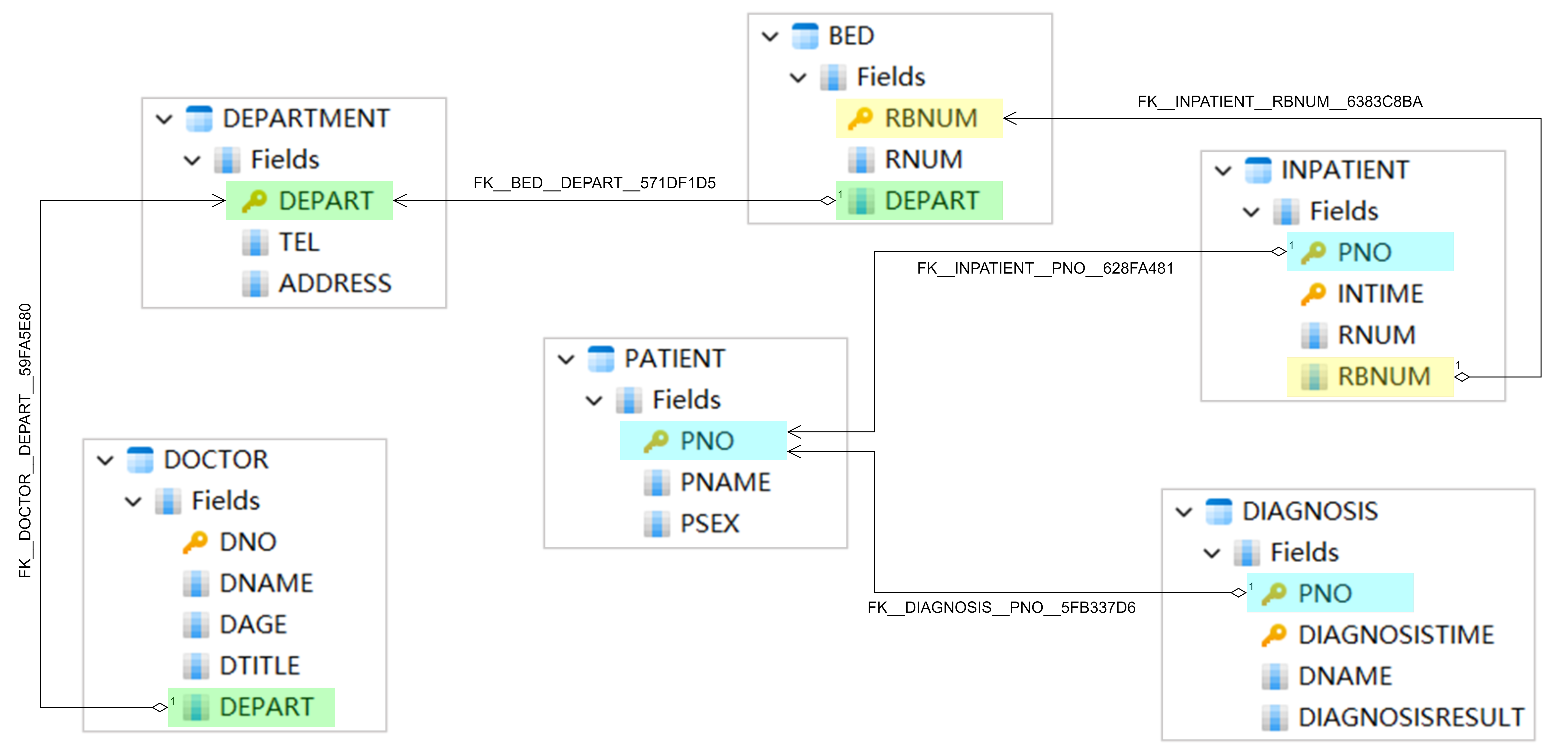
A clear visualization of table relationships, highlighting the links from Foreign Keys to Primary Keys

In the diagram provided, the arrows starting from foreign keys and ending at primary keys indicate how tables are interlinked and how SQL join queries are executed. For instance, to gather information about patients, including their names, genders, and diagnoses, seen by a specific doctor during a specific timeframe, one must focus on the field PNO, linking the DIAGNOSIS table with the PATIENT table. For readers well-versed in SQL, this type of table join query is undoubtedly a familiar sight.

This initial table structure design also has its imperfections. For example, in the DIAGNOSIS table, the doctor's name DNAME is recorded instead of their unique identifier, DNO. This design flaw results in a missing foreign key, hindering the DIAGNOSIS table from establishing a connection with the DOCTOR table to obtain detailed doctor information. Although remedial approaches could be taken by adding some common information about doctors in the DIAGNOSIS table, such as the department name DEPART, to sidestep the complexities of join queries, the challenges stemming from redundant storage, such as disk space consumption and data consistency checks, cannot be underestimated.

In the subsequent design of the graph database model, these dilemmas will no longer pose hurdles.

Let's input sample data into the aforementioned tables and amalgamate the information from all tables into a singular diagram:

Comprehensive overview of data from the 6 tables in this Hospital Information Management System

While the tabular representation, though systematic, provides a detailed and transparent overview of individual data fields, it lacks the ability to illuminate the high-dimensional interactions between data records. Questions like "which department's doctor attended to which patient" or "which patient was allocated to which ward in a specific department" are complex to deduce solely from tables. This intuitive understanding becomes notably challenging when contrasted with the forthcoming graph model we are about to construct.

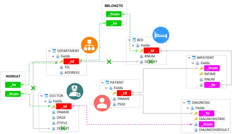
Let's begin by adopting the existing work: conceptualize each table as a schema, with the data fields serving as the properties within that schema. The challenge lies in distinguishing nodes from edges.

In essence, all tables can be likened to real-world entities, but only the most genuine entities serve as nodes. Therefore, we've identified DEPARTMENT, DOCTOR, BED, and PATIENT as nodes, utilizing their primary keys as node IDs (denoted by _id):

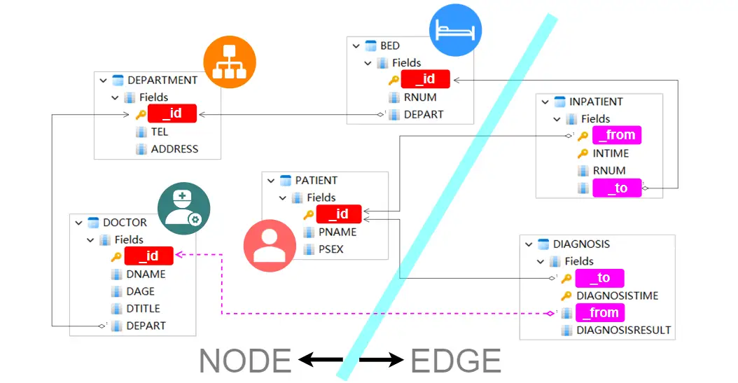
Node and Edge Differentiation

INPATIENT should not be misconstrued as a subset of PATIENT, since it captures the relationship between PATIENT and BED as evidenced by its two foreign keys. Define INPATIENT as an edge and specify its two foreign keys as the FROM and TO of the edge (denoted by _from and _to).  

(Feel free to interchange the FROM and TO of the edge as long as the edge's meaning remains coherent. For instance, setting PATIENT's _id as FROM and BED's _id as TO signifies 'patient check-in to a bed', while the reverse suggests 'bed receives a patient'.)

Applying a similar rationale, designate DIAGNOSIS as an edge to encapsulate the connection between DOCTOR and PATIENT. In determining its FROM and TO, fill in the missing foreign key linking to DOCTOR by replacing DNAME with DNO. This missing link issue was previously addressed when explaining the table structure and has now been rectified in the edge design phase.

Curious minds might wonder, "Do edges have IDs?" The answer is a resounding yes. In fact, we typically use the primary keys of tables designated as edges as their respective IDs. This logic mirrors the approach for node IDs. However, the focus isn't placed on edge IDs because, for edges, the designation of FROM and TO holds greater significance.

Two foreign keys in the original tables are still unaddressed: DEPART in the DOCTOR and BED tables, both of which link to the primary key of DEPARTMENT. This raises the question of how to handle foreign keys from tables designated as nodes.

As illustrated in the diagram below, solve these two foreign keys by introducing two new edge schemas, WORKAT and BELONGTO, which equals adding two fresh tables to the original structure:

Introducing new edge schemas WORKAT and BELONGTO

The introduction of WORKAT and BELONGTO enables the removal of the DEPART from DOCTOR and BED. As these new schemas are minimalized with only FROM and TO, additional properties can be incorporated on-demand to accommodates real-world scenarios.

Up to this juncture, all the primary keys and foreign keys in the tables are addressed. One last refinement is to isolate the RNUM field, denoting room numbers, from the BED table into a node schema ROOM, since many hospitals require calculating room occupancy or managing facilities within the room:

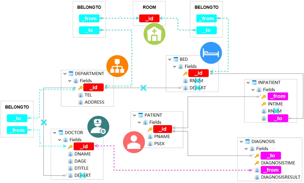
Diagram: Abstracting node schema ROOM and sharing edge schema BELONGTO

Some residual steps are: removing the redundant RNUM from both the BED and INPATIENT, sharing BELONGTO between BED-ROOM, ROOM-DEPARTMENT, and DOCTOR-DEPARTMENT since all these relationships require only properties FROM and TO.

Now cleanse and transform the tabular data into graph data in alignment with the above established graph model. Assuming each table's data is stored as an individual CSV file (e.g., DOCTOR's data saved as DOCTOR.csv) with the field names serving as headers in the file, the transformation process entails header modifications, column content replacements, and the creation of new CSV files. The detailed steps are as follows:

• In DEPARTMENT.csv, PATIENT.csv, DOCTOR.csv and BED.csv, rename headers of columns containing primary keys to '_id'.
• In IMPATIENT.csv, rename header 'PNO' to '_from', rename header 'RBNUM' to '_to', and delete the entire column 'RNUM'.
• In DIAGNOSIS.csv, rename header 'PNO' to '_to', rename header 'DNAME' to '_from', and replace the data under 'DNAME' with the corresponding data from the '_id' column in DOCTOR.csv.
• Create BELONGTO.csv with headers '_from' and '_to'.
• Copy the data under '_id' and 'DEPART' in DOCTOR.csv to '_from' and '_to' in BELONGTO.csv, ensuring the corresponding relationships of data in the same row are maintained. Then, delete the entire 'DEPART' column in DOCTOR.csv.
• Create ROOM.csv with header '_id'. Copy the unique values under 'RNUM' in BED.csv to the '_id' column in ROOM.csv.
• Copy the data under '_id' and 'RNUM' in BED.csv to '_from' and '_to' in BELONGTO.csv, ensuring the corresponding relationships of data in the same row are maintained.
• Copy the unique combined values under 'RNUM' and 'DEPART' in BED.csv to '_from' and '_to' in BELONGTO.csv, ensuring the corresponding relationships of data in the same row are maintained. Then delete the entire 'RNUM' and 'DEPART' columns in BED.csv.

As a reminder, it may be necessary to process primary keys to ensure that their associated IDs are unique[2] throughout the entire graph. Even though this doesn't apply to the data presented in this article, it is a common challenge encountered by numerous users.

Multiple approaches are available to import graph data into a designated graphset within the Ultipa graph system. Such as upload CSV files individually through Ultipa Manager, a user-friendly visualization tool for managing the Ultipa Graph system, or bulk import all files at once via the command-line utility, Ultipa Importer.

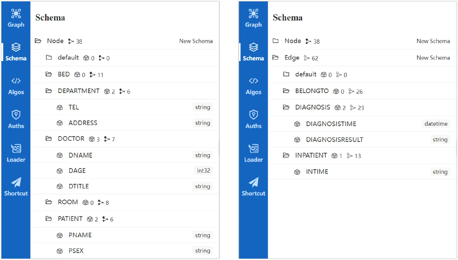
Graph model illustrated as schemas and properties in Ultipa Manager

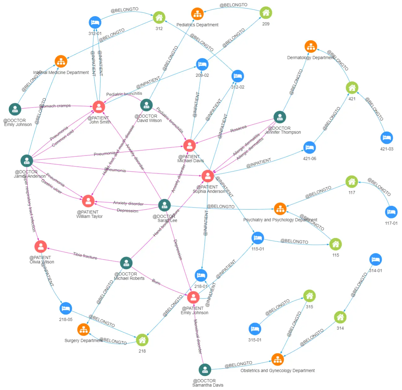
2D visualization of graph data in Ultipa Manager

Ultipa Manager's 2D rendering feature utilizes vibrant colors and icons, ensuring that relationships between different entities are distinctly visible. A quick glance allows easy identification of the interconnected nodes in the graph. This intuitive and convenient visualization sets graph databases apart, surpassing the capabilities of traditional relational databases. It greatly enhances the ease and pleasure of data analysis and exploration.

We trust this article has provided valuable insights into graph modeling, especially for newcomers venturing into the world of graph databases. In practical scenarios, constructing graph models involves more intricate situations. On the other hand, the graph model itself is not fixed, adaptable modifications are required to meet the changing business needs all the time. 

Notes:

[1] Schema: In certain relational databases like MySQL or PostgreSQL, the hierarchical data management structure within a server connection is defined as 'database-schema-table-field'. In Ultipa graph systems, this translates to 'graph-schema-property', where a schema in the Ultipa graph system corresponds to a table in relational databases, and schema properties are akin to table fields.

[2] In Ultipa, node IDs possess global uniqueness throughout the entire graph, not confined to a specific schema. For instance, if 'abc' is the ID for a particular doctor, it cannot be used as the ID for any patient or any other node within the same graph. Conversely, primary keys in relational databases only require uniqueness within their respective tables, allowing different tables to have duplicate primary keys. Consequently, certain primary keys need additional processing before they can be utilized as IDs for graph data, so do associated foreign keys.